RipStik acceleration
This term tight time frames did not leave enough time for multiple runs or practice runs. Based on recommendations from spring 2016 I went with a 100 cm interval to 800 cm. In this way I was mimicking the RipStik acceleration run of fall 2015. An attempt to keep the first 100 cm over 1.29 seconds left me unstable, I never fully recovered and lost balance post 800 cm. There was insufficient time for a second run, perhaps more time ought to be devoted to this, but the lack of time was due to review coverage of the Friday quiz. Perhaps that coverage could be reduced to provide more time for multiple runs on the sidewalk, then the smoothest run could be chosen.
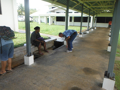
Zero was at the post next to the intersection, above I am marking 100 cm

The marks for 100 cm and 200 cm. Perhaps there is a need to try to the monotonically increasing distance model: 0, 100, 300, 700, 1200. The catch is that the sparcity of the points could lead to loss of the sense of a parabolic curve. Perhaps a 50 cm timing mark is possible, but I doubt it. The first 100 cm is eaten up trying to stabilize on a slow board.

800 cm mark.

I had no idea my camera could shoot "slow motion" but the student I passed the camera to apparently did and set the image rate to 80 frames per second. The result is the run in slow motion, including the false start. Brilliant!

Recording data.

There was a "double tap" at 200 cm and I missed either 800 or 900 cm, arguing for more space at that point between timing lines.

Data and analysis
Again there was unsteadiness in my acceleration, with an apparent loss in speed from 200 to 300 cm.

Transforming the time variable to convert the quadratic relationship to a linear relationship yields:
This suggests an acceleration of roughly 20 cm/s², which is below historic levels of 50 cm/s². Leaving time for some practice runs is a must.

The transformed data is roughly linear. Still usable for the purposes of the course, but could be better.

Zero was at the post next to the intersection, above I am marking 100 cm

The marks for 100 cm and 200 cm. Perhaps there is a need to try to the monotonically increasing distance model: 0, 100, 300, 700, 1200. The catch is that the sparcity of the points could lead to loss of the sense of a parabolic curve. Perhaps a 50 cm timing mark is possible, but I doubt it. The first 100 cm is eaten up trying to stabilize on a slow board.

800 cm mark.

The starting point. After falling off the too slow board, I obtained data during a second run.
I had no idea my camera could shoot "slow motion" but the student I passed the camera to apparently did and set the image rate to 80 frames per second. The result is the run in slow motion, including the false start. Brilliant!

Recording data.


Data and analysis
| 021 Constant Velocity | |||
| time (s) | distance (cm) | velocity (cm/s) | acc (cm/s²) |
| 0 | 0 | ||
| 2 | 100 | 50 | |
| 3.46 | 200 | 68 | 12.67 |
| 4.98 | 300 | 66 | -1.78 |
| 6.02 | 400 | 96 | 29.20 |
| 6.73 | 500 | 141 | 62.95 |
| 8.63 | 800 | 158 | 8.97 |
Again there was unsteadiness in my acceleration, with an apparent loss in speed from 200 to 300 cm.

Transforming the time variable to convert the quadratic relationship to a linear relationship yields:
| Time squared divided by two | |
| time²÷2 (s) | distance (cm) |
| 0 | 0 |
| 2 | 100 |
| 5.9858 | 200 |
| 12.4002 | 300 |
| 18.1202 | 400 |
| 22.64645 | 500 |
| 37.23845 | 800 |
| slope | 20.3661226 |
| intercept | 42.30782786 |
This suggests an acceleration of roughly 20 cm/s², which is below historic levels of 50 cm/s². Leaving time for some practice runs is a must.

The transformed data is roughly linear. Still usable for the purposes of the course, but could be better.


Comments
Post a Comment