Linear Velocity of a RipStik, Students, and Rolling Balls
I opened the week on linear velocity with the introduction of a blank time versus distance graph on the board. Then I used the LRC to F2 sidewalk to roll off a 202 cm/s run over a 3000 cm course.

I shared the data and made a sketch graph at the end of class on Monday.
Wednesday I used the Monday data to distinguish between an average and instantaneous velocity. Then I had the students measure their walking speed. I placed paper strips at the LRC and had the students walk from A101 to LRC and back, a 24200 cm round trip which was timed. The students ranged from around 90 cm/s up to around 120 cm/s.
Thursday I went with the rolling ball approach, fixed distances, and the diagonal table layout. I passed out a diagonal data entry sheet at the start of class to guide the students.

The first run, the "slow" ball run, was attempted at 100 cm increments out to 1000 cm. The fiberglass tape measure has made measurements so much easier. White chalk marked 100 cm increments, blue was 200 cm, and orange was later used for 400 cm increments.

The 8:00 lab class rolled the slow ball to 1000 cm, as did the 11:00 class. The medium speed ball was rolled out to 2000 in the 8:00 section and 1000 in the 11:00 section. An unusual south wind picked up by 11:00 and made the start more difficult.

At 8:00 Kenoma and Trisden handled the bowling task, with Trisden bowling a 796 fast ball to my best of around 444 cm/s in the 11:00 section. Ray, Gayshalane, and Philbert look on in the above shot as the ball rolls down the sidewalk.

Trisden lets loose a fast ball in the 700 cm/s range. He was accurate and generated more speed than I could.

Kenoma also proved fast and accurate from the line.


On the fast runs with 400 cm increments out to 2400 cm, the timers could not well see the chalk marks. I realized the key would be to put people on the marks and the timers could cue off of the people. Michelle on the left, Diane, Nagsia, Beverly, and Glenn at the far end mark 400 cm increments. I was bowling.

Vandecia took over from Michelle.
Up in the lab I demonstrated the optional use of Google Docs to build lab reports for the first time. Noting that a trend line cannot be displayed on an xy scatter graph, I built a second table.

That second table can be seen above with the orange header. Note the diagonal data arrangement. This permits three lines with differing x-values to appear on a single xy scatter graph in a spreadsheet. Above is Google Sheets.
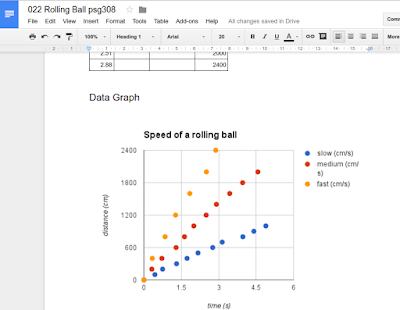
Google Sheets now supports graphs in documents, and the graphs remain linked to the original in Sheets.


I shared the data and made a sketch graph at the end of class on Monday.
Wednesday I used the Monday data to distinguish between an average and instantaneous velocity. Then I had the students measure their walking speed. I placed paper strips at the LRC and had the students walk from A101 to LRC and back, a 24200 cm round trip which was timed. The students ranged from around 90 cm/s up to around 120 cm/s.
Thursday I went with the rolling ball approach, fixed distances, and the diagonal table layout. I passed out a diagonal data entry sheet at the start of class to guide the students.

The first run, the "slow" ball run, was attempted at 100 cm increments out to 1000 cm. The fiberglass tape measure has made measurements so much easier. White chalk marked 100 cm increments, blue was 200 cm, and orange was later used for 400 cm increments.

The 8:00 lab class rolled the slow ball to 1000 cm, as did the 11:00 class. The medium speed ball was rolled out to 2000 in the 8:00 section and 1000 in the 11:00 section. An unusual south wind picked up by 11:00 and made the start more difficult.

At 8:00 Kenoma and Trisden handled the bowling task, with Trisden bowling a 796 fast ball to my best of around 444 cm/s in the 11:00 section. Ray, Gayshalane, and Philbert look on in the above shot as the ball rolls down the sidewalk.

Trisden lets loose a fast ball in the 700 cm/s range. He was accurate and generated more speed than I could.

Kenoma also proved fast and accurate from the line.

Francina on tape line anchor and ball retrieval


Vandecia took over from Michelle.
Up in the lab I demonstrated the optional use of Google Docs to build lab reports for the first time. Noting that a trend line cannot be displayed on an xy scatter graph, I built a second table.

That second table can be seen above with the orange header. Note the diagonal data arrangement. This permits three lines with differing x-values to appear on a single xy scatter graph in a spreadsheet. Above is Google Sheets.

Google Sheets now supports graphs in documents, and the graphs remain linked to the original in Sheets.

A second table is necessary in Google Sheets to report the slopes (speeds) and intercepts. Schoology as a Google Drive add on that allows direct submission of Google Docs. I am unclear exactly why I would return to Excel, and even LibreOffice.org loses some of its luster against a suite that can run on my cell phone if the need were to arise.
The basic approach of rolling the ball past fixed distances that are increased with increasing velocity worked well enough. The issue of the first second being faster dates back in the earliest days of my taking over the course. The set-up used for a number of years can be seen in a 2008 photo sequence. The loss of speed after the first second was more pronounced when the parking lot was wet or littered with leaves and sticks. Yet moving to the slick tile of the gym porch still did not eliminate the speed drop after the first second.
Although I was deeply attached to keeping the time as the independent variable and the distance as the dependent variable (hence students attempting to note the position of the ball at an assigned second), ultimately years of tinkering could not remove the pseudo-speed loss that reaction times were introducing. For some reason, measuring time to fixed distances produces a more linear relationship with no significant speed fall off after the first second.
The lab has also forgone graphing the slope zero, speed zero ball, in favor of three moving balls, slow, medium, and fast. The zero slope case is mentioned, but no longer graphed.
Comments
Post a Comment