Acceleration, energy, and momentum

For the introduction of accelerated motion in SC 130 Physical Science I utilized the longer 90 minute summer periods and did the RipStik acceleration in the parking lot.



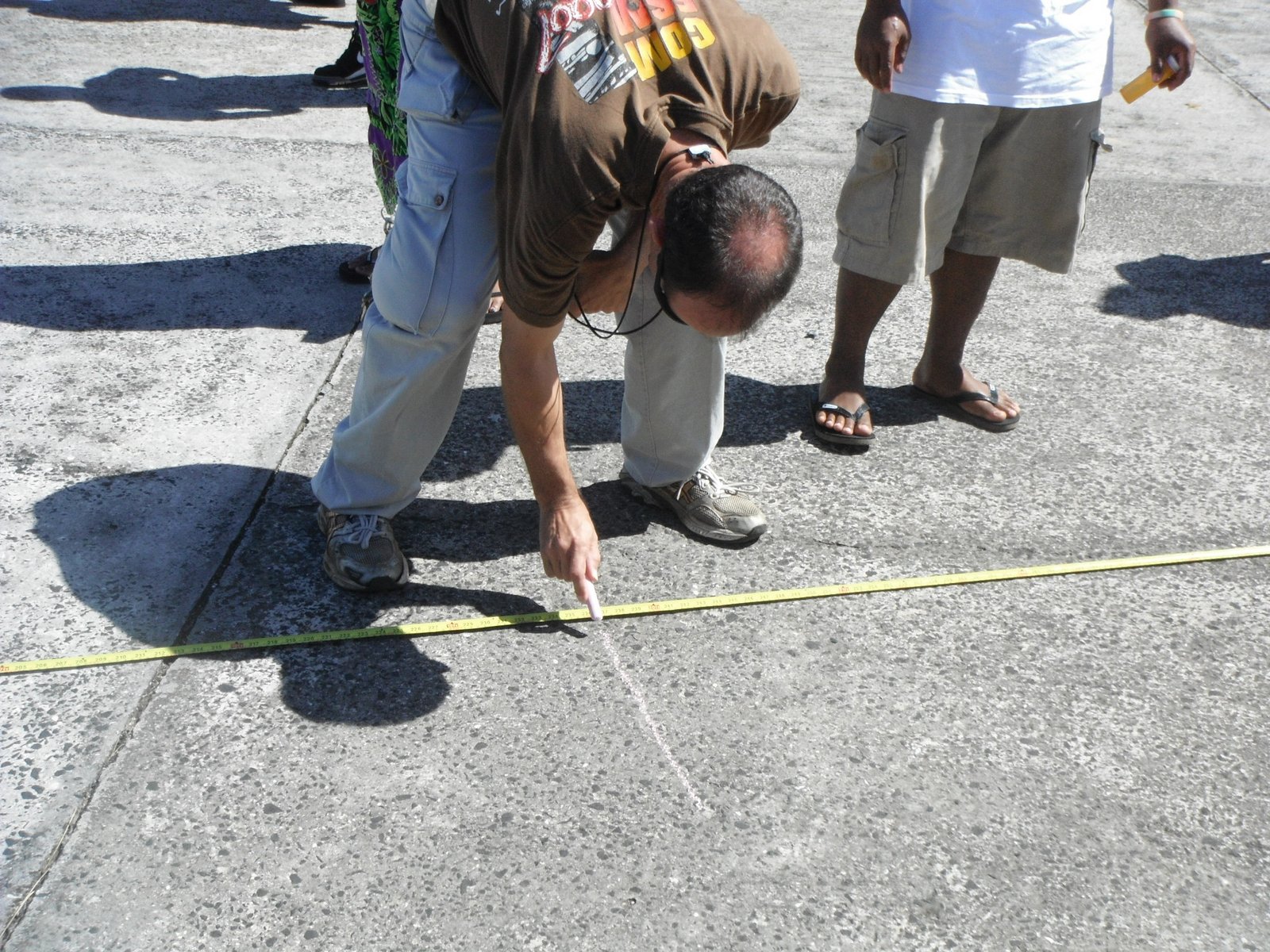
I placed chalk marks every 200 cm for the first 800 cm using an 800 cm tape measure.



Then I spaced the marks every 400 meters for the second 800 cm.



This seemed to work reasonably well, although I finished the run with as much speed as I am comfortable generating. I had to burn speed on an uphill carving turn. I carried the stopwatch in my right hand, passing off my keys and camera to the students.



I used a diagonal run to take advantage of the natural slope. I also pumped the board.









The data was recorded on the white board and graphed. A rough graph showed a strong positive curvature to the acceleration data on a time versus distance graph.




The right board includes parts of the pre-RipStik run introduction to accelerated motion. The marbles last week had slowed down significantly on the table, leading to negative curvature on time versus distance charts.



In the afternoon the students dropped super balls on the way to determining the acceleration of gravity g in laboratory 032. Beverleen holds the meter sticks, Judy drops the ball and times.



Gasma, Arnold, and Melyda gather data.



Kramwel and Johnson use the wall to support their meter sticks.



Tommy drops the ball while Rosalina holds the meter stick. Laurie records their data.



Isinta drops and times, May-vy steadies the meter stick.



On Wednesday morning I opted to use the Hot Wheels car and track for the non-linear model. I use the lecture in part to give the non-science majors in the class a taste of physics. I start by noting that for a height of zero the speed of the car at the bottom of the ramp is zero. Then I let the car roll from a height of 10 cm and time the car over a distance of 100 cm on the table. I then stop and ask the students to predict the speed from 20 cm. Invariably someone guesses that the speed will double, and this become the "linear prediction."



As the height increases and the speed measurements accumulate, it becomes increasingly evident that a linear model overestimates the car speed. A graph of the linear prediction and actual speed shows that the actual speed does have a pattern. There is a smooth curve. And a smooth curve means that there exists a mathematical model.



I then introduced the idea of conservation of energy, gravitational potential energy, and kinetic energy. During the regular term I have the opportunity to do the RipStik on Monday and to introduce these concepts. I did not have time to do that ahead of the Hot Wheels car drop on the ramp.

I hung the ramp from the overhead track, tying it to the rail with string.


Isinta and Beverleen time their marble.

I also modified laboratory 042. I ran the mass in equals mass out without the focus on the penultimate marble. With the class observing I generated the unit slope graph. Then I had the students work by table in measuring speed in versus speed out using two stopwatches. I encouraged the use of long tracks.


Gasma, Arthy, and Arnald

The use of two timers and longer tracks made the measurements conceptually easier. The groups were less confused and fewer groups tried to use the "on slope" time.


Tommy times while Laurie observes.



I built an odd track using two long triangular paper tubes. The effort was a failure - the outbound marbles had only 46% of the speed of the inbound marble - larger speed losses than Tommy was getting from his ruler track rig.

Ultimately short outbound distances may be important due to frictional issues.