Converting Likert survey words in Google Forms to numbers in Google Sheets
In Google Forms a multiple choice grid such as the above generates a spreadsheet that has the word responses. The following looks at converting these word values to numbers allowing for statistical analysis.
The first tab will be Form Responses 1. Do not edit this sheet. This is the sheet on which results arrive, with results being appended below the last row of the spreadsheet. Altering or working directly in this sheet is not recommended.
Instead, add a new tab. In the above the tab is labelled d for data. The label is arbitrary but shorter and simpler will be easier to work with later on. Spaces can be particularly problematic in later formulas requiring extra quotation marks.
The function being used is the IFS formula, essentially a variation of a CASE statement in other languages. IFS replaces nested IF functions. The function in A2 is pulling the value in H2 from the Form Responses 1 spreadsheet. The function in A2 is:
=IFS('Form Responses 1'!H2="Strongly disagree",1,'Form Responses 1'!H2="Disagree",2,'Form Responses 1'!H2="Neutral",3,'Form Responses 1'!H2="Agree",4,'Form Responses 1'!H2="Strongly agree",5,'Form Responses 1'!H2="Not applicable","")
Note that if the form is still open for responses, then the formula will have to be filled down further as new responses appear on the Form Responses 1 tab. This function can be adapted to handle any multiple choice word responses. In this instance the formula is assigning the values 1 to 5 for strongly disagree to strongly agree. Nothing else is happening on this tab.
The third tab is the a tab for analysis. The function in A2 calculates the average in column A of the d tab. This formula was filled right to generate averages for each column. Similar structures can be used to obtain the count (sample size), mode, median, and - if deemed meaningful - the standard deviation. Other calculations can be made at this point as appropriate to the nature of the data being collected.
The colors seen are the result of using conditional formatting and a color scale with values set appropriate to the data set. The midpoint may need adjusting or can be set to a percent or percentile to adjust more automatically.
Because respondents tend to choose 4 or 5, a highly modified form of a z-score is used in A5 above to produce charts that help display when a mean is perhaps unusual. The value in AB is the mean of the means in that section of the survey, in AC is the standard deviation of the means for that section of the survey. Being a spread of the means themselves, not the underlying data, this is perhaps related to the standard error of the mean, but it is not the standard error of the mean. The large sample size and the presence of the square root of that sample size in the denominator of the denominator generates large t-statistics that are not particularly informative.
The result can be a chart such as the above, with values beyond ±2 highlighted as areas of relative weakness and relative strength.
Other functions can also be deployed to directly tally word responses when the number of word responses are few. Above a COUNTIF function is deployed to tally options found in column E on the Form Responses 1 listed in column AV.
=COUNTIF('Form Responses 1'!E:E,AV2)
In the above formula the E:E reference is used to include all rows in Form Responses 1, especially useful if the form is still open and rows are being added. Note that in the above screenshot row 4 is not being displayed.
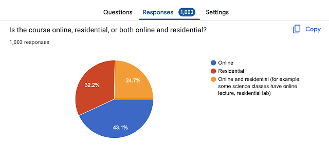
The results can then be displayed as a chart.
Although, to be fair, this chart is also available directly from the Responses tab. Still, there are more chart options available when working from Google Sheets.
There are many approaches to converting words to numbers including good old fashioned find and replace. Find and replace, however, has to be run every time new data arrives. The above system just requires filling down a function in tab d to pick up the newly arrived response rows. This is easier and faster than running the six find and replace operations.
Other approaches would be to use COUNTIF to get counts of the numbers in each column and then use those counts to calculate a column mean using a weighted average. For extremely large spreadsheets perhaps the COUNTIF approach would be more efficient. In the above there are 25,075 IFS functions operating.
Using COUNTIF and a weighted mean would require the use of perhaps 60 functions. Each column would need five COUNTIF functions, there are ten columns. There would then need to be ten weighted mean functions.
There may be some advantages to the use of IFS over COUNTIF. A column can added to the d tab to calculate the standard deviation of each row. Standard deviations of zero represent a response set that is a "straight ticket" - the respondent has marked all responses with the exact same value. That suggests the respondent may not have been actually reading and responding to prompts. In a prior run of the survey 44% of the respondents had marked a straight ticket.


Comments
Post a Comment