Soap density and RipStik linear velocity
Summer term in SC 130 physical science is always compressed. Monday the preassessment was run, only the ability to plot data values in a table on an xy scatter graph exceeded a 70% success rate. At just under 70% was the ability to determine the slope and intercept when given a line on a graph and correctly identifying the y-intercept when given an equation in the form y = b + mx. Monday wrapped up with a move to the computer laboratory to get the students logged into Schoology. The A204 lab was unscheduled from 9:30 to 11:00 this summer. Having at least one period of lab access is very useful to the SC 130 physical science course.

Tuesday the preassessment was reviewed. The students used a tape measure and scale to determine their height in meters, their mass in kilograms, and their body mass index. Short of the end of the period the two students who had been absent Monday were taken upstairs to get logged into the course.
Wednesday morning the students worked out the density of seven masses, then I led a demonstration of the density of water.

The afternoon was occupied with the density of soap laboratory. Using graph paper each pair graphed their data, manually determined their slope, used that to predict float/sink, and then tested their soap. This went rather well, perhaps because this is the first laboratory and the students had no expectation of what a computer can do in terms of xy scatter graphs.


With the loss of the computer laboratory in summer, graphing on graph paper was deployed as an alternative.
Thursday morning I used A204 to demonstrate how to use word processors and spreadsheets to lay out a laboratory report for the class. As used Microsoft Word and Excel as that is what the students will have access to in the library. That meant that the 021 "Monday" RipStik run never happened. As I did last summer, I opted to the RipStik and lap timers.

This summer I took the distance out to 30 meters.

The full 30 meter run. For any sufficiently short distance a velocity can appear to be constant, 30 meters tests my ability to hold a constant velocity.

Seven lap timers meant 14 students could pair up as timer and data recorder pairs. I called "start, split, split, split,... stop" during the 30 meter RipStik run. The first run was perhaps a tad too fast at about 28 seconds for 30 meters (~107 cm/s). I had started up the slope. I would later start a meter shy of the 0 mark and achieve a wobbly slower speed 49 second run (~61 cm/s). I wanted to go slow to fast, so the first run has to be as slow as possible. I intentionally omitted the 0 cm/s run.

A second run was done slightly faster, taking roughly 15 seconds or about 200 cm/s over the 30 cm course. My running speed is up around 250 cm/s, so I know that I cannot jump off the board at the end of a run at much more than that.

The third run was just under 10 seconds up around 308 cm/s. The jump off was sketchy at this speed because I was landing the jump off on the down slope towards the A building. Decelerating downhill is more challenging when going from standing still on a board to 308 cm/s, at least for me.
Perhaps the trick on the third run would be to reverse the run since I am powering the run. That would let me run out uphill towards the LRC, burning off some speed before I hit the east wall of the LRC. The distances would be 0, 300, 600, 1000, 1500,...

Marmelyn and Neikaman display their data sheet.

The data sheet was prepared in advance, printed, and handed out, as the one in the text is too short for this summer version of the activity. In advance I was going to have seven rows per run, but then I tossed in three more for ten each (although the middle block above is eleven rows). I did not know what distances I would use at that time. Out on the sidewalk I rediscovered that the posts are about 300 cm apart, 305 cm actually. So I opted to use 300 cm intervals: 0, 300, 600, 900, 1200, 1500. Then there is a gap in the posts for the entrance to the south faculty building. I put a mark at 2000 which is midway along the gap, then 2400, 2700, and 3000 cm. Which was ten data values including the 0 seconds at 0 centimeters.

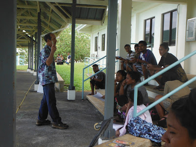
The class stayed outside on the stairs.

I then asked what was the relationship between time and distance, or more precisely, how could we determine that relationship? I then had them graph their data on a single graph. This would be followed up by a Friday morning computer lab session to show how the unique table layout translates to three lines on one spreadsheet xy scatter graph.


Preliminary results suggest reasonably linear data. I wrapped up with a demonstration of zero speed at 1500 cm and then a question and answer on what the slope would be for this situation. I also worked on leading them through the logic of a vertical line, undefined slope, being two places at one time situation.
The data seen above yielded the following charts.

The wobbly 49 second run is not on the graph. Note that adding linear regressions in Excel causes the y-axis scale to essentially double. That has to be manually reset.

The split speeds. The 581 cm/s is a timing error.

Tuesday the preassessment was reviewed. The students used a tape measure and scale to determine their height in meters, their mass in kilograms, and their body mass index. Short of the end of the period the two students who had been absent Monday were taken upstairs to get logged into the course.
Wednesday morning the students worked out the density of seven masses, then I led a demonstration of the density of water.

Sucy-ann and Marmelyn record data
The afternoon was occupied with the density of soap laboratory. Using graph paper each pair graphed their data, manually determined their slope, used that to predict float/sink, and then tested their soap. This went rather well, perhaps because this is the first laboratory and the students had no expectation of what a computer can do in terms of xy scatter graphs.

Marsha and Marlinda measure their soap

Joemar and Shirley-ann recorded data.

Dial soap data

Ivory soap data recording in the physical science text data table

Ivory soap data

John and Gino hand graphing
With the loss of the computer laboratory in summer, graphing on graph paper was deployed as an alternative.
Thursday morning I used A204 to demonstrate how to use word processors and spreadsheets to lay out a laboratory report for the class. As used Microsoft Word and Excel as that is what the students will have access to in the library. That meant that the 021 "Monday" RipStik run never happened. As I did last summer, I opted to the RipStik and lap timers.

This summer I took the distance out to 30 meters.

The full 30 meter run. For any sufficiently short distance a velocity can appear to be constant, 30 meters tests my ability to hold a constant velocity.

Seven lap timers meant 14 students could pair up as timer and data recorder pairs. I called "start, split, split, split,... stop" during the 30 meter RipStik run. The first run was perhaps a tad too fast at about 28 seconds for 30 meters (~107 cm/s). I had started up the slope. I would later start a meter shy of the 0 mark and achieve a wobbly slower speed 49 second run (~61 cm/s). I wanted to go slow to fast, so the first run has to be as slow as possible. I intentionally omitted the 0 cm/s run.

A second run was done slightly faster, taking roughly 15 seconds or about 200 cm/s over the 30 cm course. My running speed is up around 250 cm/s, so I know that I cannot jump off the board at the end of a run at much more than that.

The third run was just under 10 seconds up around 308 cm/s. The jump off was sketchy at this speed because I was landing the jump off on the down slope towards the A building. Decelerating downhill is more challenging when going from standing still on a board to 308 cm/s, at least for me.
Perhaps the trick on the third run would be to reverse the run since I am powering the run. That would let me run out uphill towards the LRC, burning off some speed before I hit the east wall of the LRC. The distances would be 0, 300, 600, 1000, 1500,...

Marmelyn and Neikaman display their data sheet.

The data sheet was prepared in advance, printed, and handed out, as the one in the text is too short for this summer version of the activity. In advance I was going to have seven rows per run, but then I tossed in three more for ten each (although the middle block above is eleven rows). I did not know what distances I would use at that time. Out on the sidewalk I rediscovered that the posts are about 300 cm apart, 305 cm actually. So I opted to use 300 cm intervals: 0, 300, 600, 900, 1200, 1500. Then there is a gap in the posts for the entrance to the south faculty building. I put a mark at 2000 which is midway along the gap, then 2400, 2700, and 3000 cm. Which was ten data values including the 0 seconds at 0 centimeters.

The class stayed outside on the stairs.

Gino and John


Neikaman graphing

Gino, John, graphing

The class working on the steps
Preliminary results suggest reasonably linear data. I wrapped up with a demonstration of zero speed at 1500 cm and then a question and answer on what the slope would be for this situation. I also worked on leading them through the logic of a vertical line, undefined slope, being two places at one time situation.
The data seen above yielded the following charts.

The wobbly 49 second run is not on the graph. Note that adding linear regressions in Excel causes the y-axis scale to essentially double. That has to be manually reset.

The split speeds. The 581 cm/s is a timing error.


Comments
Post a Comment