Acceleration, momentum, and pulleys
Monday class was held in MITC. The class watched the first three-quarters or so of Earth from Space. Tuesday began with a review of the linear motion of rolling balls at different velocities, laboratory two results.
 Then I moved on to note what a decelerating or accelerating ball would look like on a time versus distance graph.

I also covered a velocity of zero and returning back to a starting point - negative velocity. This was in preparation for the RipStik deceleration run on the sidewalk.

The RipStik deceleration run went surprisingly well. I did a single practice run. For the timed run I started with the same post which had been zero for laboratory two, heading west towards the LRC. I used the posts, which I found to be 305 cm center on center including the sidewalk spanning post set that I had thought was a 320 cm span. That span is apparently 305 as well.
The data went well. I did a hand calculation of a fit, and then ran a calculation on a calculator. Laboratory three, in the afternoon, then measured the acceleration of gravity.


The table seen in the text above is the older long form table seen in edition 5.1. Only 5.2 includes the newer short form table.
 Notes on board during lab period include morning notes on the left.

The construction of the soccer field on the north side of the entrance road had taken out my crop of banana leaf marble ramps. I tried using the Hot Wheel tracks, but oddly enough the data did not generate a smooth relationship.
 The point of this exercise is to show that some relationships are not linear. In this case the relationship is a square root relationship - derived from setting the gravitational potential energy energy equal to the kinetic energy. I opt to neglect rotational kinetic energy as the class is confused enough by the linear kinetic energy calculation.


The data can be seen underestimating the "44.2" theoretic curve except up at 100 cm. And the data does not leave one convinced that the correct underlying model is a square root model. Who knew - banana leaf marble ramps produce more mathematically consistent results than slick Hot Wheels tracks.

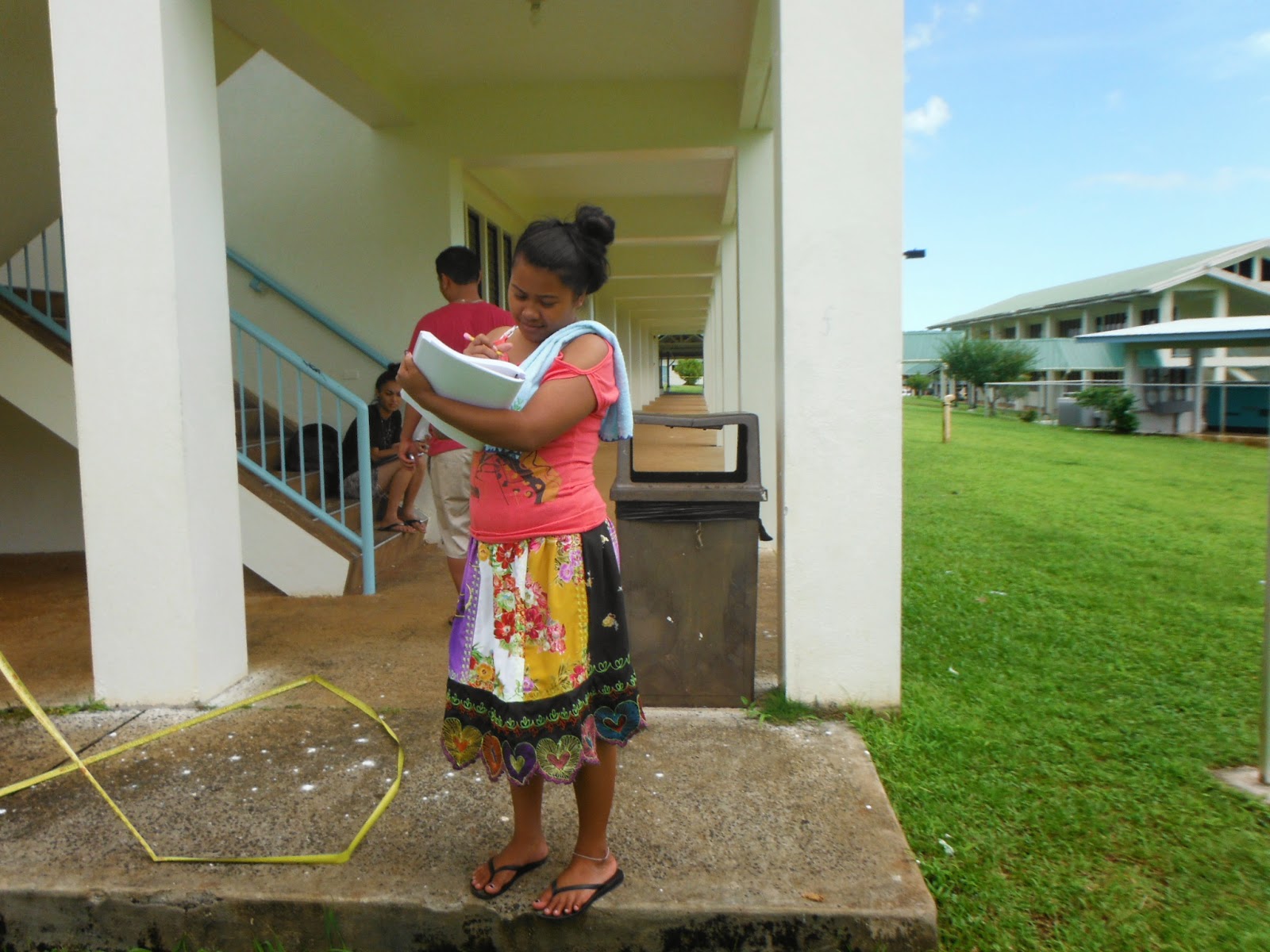
A new approach was taken to laboratory four using sheets of poster pad and circular arcs. Single duck marbles were sent into a single sitting duck marble. Aiming proved extremely problematic.

Arcs were made using lengths of yarn.

One group deployed guides for the inbound marble, which solved the aiming difficulty. The outbound speeds, however, were still significantly below the inbound speeds. Momentum losses were large - over 50%, all in the loss of velocity. The source of the loss may in part be inelasticity, but that is probably the least of the losses. The largest "loss" is that the inbound marble rarely comes to a complete stop - some momentum is left in the inbound marble. There are also losses in the spin down of the inbound marble, spin up of the outbound marble. The outbound marble also loses speed with distance, although one group used their arcs at 10 cm, 20 cm, 30 cm, 40 c, and 50 cm to measure ever increasing outbound distances. This seems to have offset some of the velocity loss seen in the slower marbles (slower marbles were measured over shorter distances).
Thursday's lecture on Newton's three laws used the RipStik and a rolling ball on lined up tables to illustrate the laws. This makes a good lecture demonstration of relative velocity and frames of reference. The pulley lab was unchanged from prior terms.

A momentum data sheet from Wednesday.


Notes from Newton.
 As always these are only notes to myself and provide guidance to any future run of the course I might handle. The intended reader is only the future me.
I also covered a velocity of zero and returning back to a starting point - negative velocity. This was in preparation for the RipStik deceleration run on the sidewalk.
The RipStik deceleration run went surprisingly well. I did a single practice run. For the timed run I started with the same post which had been zero for laboratory two, heading west towards the LRC. I used the posts, which I found to be 305 cm center on center including the sidewalk spanning post set that I had thought was a 320 cm span. That span is apparently 305 as well.
The data went well. I did a hand calculation of a fit, and then ran a calculation on a calculator. Laboratory three, in the afternoon, then measured the acceleration of gravity.
 |
| Charlotte |
 |
| Pamela |
The table seen in the text above is the older long form table seen in edition 5.1. Only 5.2 includes the newer short form table.
The construction of the soccer field on the north side of the entrance road had taken out my crop of banana leaf marble ramps. I tried using the Hot Wheel tracks, but oddly enough the data did not generate a smooth relationship.
The data can be seen underestimating the "44.2" theoretic curve except up at 100 cm. And the data does not leave one convinced that the correct underlying model is a square root model. Who knew - banana leaf marble ramps produce more mathematically consistent results than slick Hot Wheels tracks.
A new approach was taken to laboratory four using sheets of poster pad and circular arcs. Single duck marbles were sent into a single sitting duck marble. Aiming proved extremely problematic.
Arcs were made using lengths of yarn.
One group deployed guides for the inbound marble, which solved the aiming difficulty. The outbound speeds, however, were still significantly below the inbound speeds. Momentum losses were large - over 50%, all in the loss of velocity. The source of the loss may in part be inelasticity, but that is probably the least of the losses. The largest "loss" is that the inbound marble rarely comes to a complete stop - some momentum is left in the inbound marble. There are also losses in the spin down of the inbound marble, spin up of the outbound marble. The outbound marble also loses speed with distance, although one group used their arcs at 10 cm, 20 cm, 30 cm, 40 c, and 50 cm to measure ever increasing outbound distances. This seems to have offset some of the velocity loss seen in the slower marbles (slower marbles were measured over shorter distances).
 |
| Maria-Asunscion |
Thursday's lecture on Newton's three laws used the RipStik and a rolling ball on lined up tables to illustrate the laws. This makes a good lecture demonstration of relative velocity and frames of reference. The pulley lab was unchanged from prior terms.
A momentum data sheet from Wednesday.
 |
| Charlotte |
 |
| Emmy Rose |
Notes from Newton.


Comments
Post a Comment