Thermal conductivity and mathematical models
An attempt to build on last term's note, "I fiddled and tweaked my way to the initial logistic expression by using
a computer in the possession of Brinando and Megan. They watched as I
fumbled and fought my forward to a design that would behave in a way
similar to their data. I explained what I was doing and why, including
referring to the (x - h) portion of the graph. I gather one or both had
MS 101 Algebra and Trigonometry, so they were not necessarily completely lost in my
ramblings. I thought that interchange was valuable, that exercise was
valuable. They were able to see their instructor struggle with a
mathematical model, not have it quite right at first, and then iterate
his way to a reasonable solution," did not go as well as hoped in the 8:00 lab.
I did not use a lap top as I did in the fall. Note two that all but one group saw an immediate and rapid linear rise in temperature until the peak temperature was reached. Only one group had that characteristic initial "flat" segment. My only thought for 11:00 is to attempt to get some temperature readings in the first minute, maybe at 30 seconds. I think I might also drag along my lap top and use that to chart the data.

At 11:00 I used the lap top and began on a 30 second timing. Even with this a couple groups had no initial "flat" segment - by 30 seconds the temperature was already rising. Using the lap top I was able to finesse the equation, but ultimately this did not lead to anything more than "sometimes you can see things you do not understand from a mountaintop."
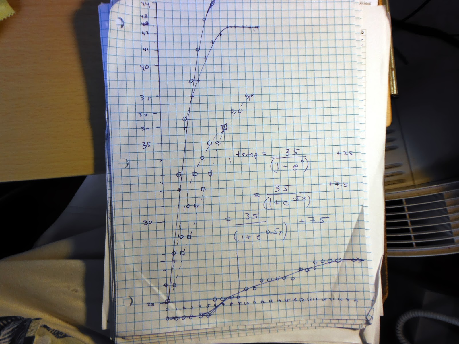
 The function is a logistic function, but not in a probability format. The starting structure is essentially (y - k) = range/(1-e^(-a(x-h))) where k is the start value and h is the x-value at the middle of the rise in temperature. Note that for some groups the best fit is achieved by calling (0, 25) the middle of the rise i temperature. This puts the theoretic start value at 25-(maximum-25), if 25 is the start value. I know that can be reduced, but then the meaning is lost.

Ideally the system holds at the starting temperature, then the range is the vertical span of the logistic function.
The coefficient a is found by trial and error, this affects the speed of the rise. Values of 0.6 to 0.8 appear to generate best fits. The actual function in spreadsheet cell C2 is =F$3/(1+EXP(-F$8*(A2-F$7)))+F$1 where F$3 contains the vertical range, F$8 contains the coefficient, F$7 contains the midrise time, and F$1 contains the start value. A2 holds the time.
I did not use a lap top as I did in the fall. Note two that all but one group saw an immediate and rapid linear rise in temperature until the peak temperature was reached. Only one group had that characteristic initial "flat" segment. My only thought for 11:00 is to attempt to get some temperature readings in the first minute, maybe at 30 seconds. I think I might also drag along my lap top and use that to chart the data.
At 11:00 I used the lap top and began on a 30 second timing. Even with this a couple groups had no initial "flat" segment - by 30 seconds the temperature was already rising. Using the lap top I was able to finesse the equation, but ultimately this did not lead to anything more than "sometimes you can see things you do not understand from a mountaintop."
Ideally the system holds at the starting temperature, then the range is the vertical span of the logistic function.
The coefficient a is found by trial and error, this affects the speed of the rise. Values of 0.6 to 0.8 appear to generate best fits. The actual function in spreadsheet cell C2 is =F$3/(1+EXP(-F$8*(A2-F$7)))+F$1 where F$3 contains the vertical range, F$8 contains the coefficient, F$7 contains the midrise time, and F$1 contains the start value. A2 holds the time.


Comments
Post a Comment