From longitude to spectra
Finding Binky went rather well on a Wednesday morning. In the afternoon I opted to deploy the redesigned laboratory seven. The new design once again simplifies a laboratory that has continued to remain confusing for the students. The redesign puts a linear relationship into the core of the laboratory, including a graph.
In retrospect I should have simply subtracted the starting longitude. The class walked east on a line of latitude. Not "zeroing" the longitude data leads to a large and rather meaningless y-intercept. Future runs should deduct the starting longitude when walking along a line of latitude.

I chose to roll the surveyor's wheel while the students held the GPS units. The surveyor's wheel is not zeroing properly any longer and I did not want to potentially introduce errors due to misreading the surveyor's wheel counter. Every 100 feet I had the students report their longitude value. These distances were logged at "30 meters" rather than the 30.48 meters they actually are. Teh difference is 1.6%. They also worked to ensure I remained on the same line of latitude.
The day was damp and threatening rain, so I started from in front of the prep room. This would prove to be a sub-optimal choice, eventually generating only four data coordinates by the time we had crossed the road and hit private property. Starting back at the main lot is highly recommended.

The data turned out to be highly linear and was within 1.7% of the actual value - coincidentally close to the known error. The students remained confused about what we had measured and whether we had measured minutes of longitude or latitude. That said, this simplification brought understanding closer. Tossing the meter measurements done with the GPS units and returning to a two variable xy scattergraph relationship aligns the lab with the redesigned lab five on pulleys and lab nine sound speed lab. All three now generate linear relationships with slopes.
Laboratory eight led off with cloud watching and moved into a drawing session. I was surprised by the group's general enthusiasm for drawing. The lab went almost to two o'clock.


For the introduction of waves done in 091 I realized that the uphill on the walkway would force a more aggressive sine wave swizzle with my RipStik. This was indeed the case. I also chose to use three sheets of paper which gave me 250 cm to work with.

I then ran calculations on a poster board. I had managed to lay down 7 wavelengths in 2.22 seconds. I used the language "wiggles" and first asked the students to count the wiggles. Of his own volition one student counted only crests and not troughs, the class concurred with his count. This made explaining wavelength easier.
The wavelength dropped as I moved uphill from about 40 cm to around 32 cm. 250 cm/7 waves provided an average wavelength of 35.7 cm. The frequency was 7 wiggles in 2.22 seconds or 3.15 Hz - one the highest frequencies I can recall. 3.15 * 34.7 yielded a wave speed of 112 cm/s. The board speed of 250 cm/2.22 s is also 112 cm/s rounded off. Done this way the underlying identity is hidden and the result looks magical. The wave speed is the board speed.

In the afternoon I managed to get a spot on velocity in laboratory nine by using the berm as a back shield to pick off a faint echo from the book store at a location record of 224 meters. The day was extremely hot and sunny, the class was melting, and I was feeling energetic that day.

The gym echo was tougher to synch on, so one student tried to time a single echo. The results were off. The error appears to have been 0.2 seconds, enough to significantly undervalue the speed the of sound. There is a reaction time issue between a clapper and timer. I recommended that the class not use the four values at one second and 300 meters.

Nice cirrus appeared late in the evening on the way to the parking lot.

Laboratory ten remains the odd child out. The loss of the computer lab and the RGB color focus leaves the lab at loose ends. Continuous spectra led the lab. All images were acquired using CD spectrometers in boxes. I simply stuck the camera up to the eyehole and shot on auto.

The I moved on to spectra tubes. Above one line from hydrogen is simply missing - the camera sensor is insensitive to that one wavelength.

Mercury had a golden line that was green in the raw camera image. Auto-balancing the image in GIMP restored the golden line.

Mercury displaying many pairs of red lines, a pair of yellow lines (color distorted above), a pair of orange lines, and a pair of faint green lines.
I showed the students the camera images and used the inability of the camera to image some light bands as a starting off point for a lecture on the subtleties of color perception. Somewhere in there is a laboratory struggling to get out.
In retrospect I should have simply subtracted the starting longitude. The class walked east on a line of latitude. Not "zeroing" the longitude data leads to a large and rather meaningless y-intercept. Future runs should deduct the starting longitude when walking along a line of latitude.

I chose to roll the surveyor's wheel while the students held the GPS units. The surveyor's wheel is not zeroing properly any longer and I did not want to potentially introduce errors due to misreading the surveyor's wheel counter. Every 100 feet I had the students report their longitude value. These distances were logged at "30 meters" rather than the 30.48 meters they actually are. Teh difference is 1.6%. They also worked to ensure I remained on the same line of latitude.
The day was damp and threatening rain, so I started from in front of the prep room. This would prove to be a sub-optimal choice, eventually generating only four data coordinates by the time we had crossed the road and hit private property. Starting back at the main lot is highly recommended.

The data turned out to be highly linear and was within 1.7% of the actual value - coincidentally close to the known error. The students remained confused about what we had measured and whether we had measured minutes of longitude or latitude. That said, this simplification brought understanding closer. Tossing the meter measurements done with the GPS units and returning to a two variable xy scattergraph relationship aligns the lab with the redesigned lab five on pulleys and lab nine sound speed lab. All three now generate linear relationships with slopes.
Laboratory eight led off with cloud watching and moved into a drawing session. I was surprised by the group's general enthusiasm for drawing. The lab went almost to two o'clock.

Jane Rose Peter and Tracy Donre study cloud pictures.

Rose Ann Letawigemal and Risenta Cholymay

Jane Rose and Tracy at work.

For the introduction of waves done in 091 I realized that the uphill on the walkway would force a more aggressive sine wave swizzle with my RipStik. This was indeed the case. I also chose to use three sheets of paper which gave me 250 cm to work with.

I then ran calculations on a poster board. I had managed to lay down 7 wavelengths in 2.22 seconds. I used the language "wiggles" and first asked the students to count the wiggles. Of his own volition one student counted only crests and not troughs, the class concurred with his count. This made explaining wavelength easier.
The wavelength dropped as I moved uphill from about 40 cm to around 32 cm. 250 cm/7 waves provided an average wavelength of 35.7 cm. The frequency was 7 wiggles in 2.22 seconds or 3.15 Hz - one the highest frequencies I can recall. 3.15 * 34.7 yielded a wave speed of 112 cm/s. The board speed of 250 cm/2.22 s is also 112 cm/s rounded off. Done this way the underlying identity is hidden and the result looks magical. The wave speed is the board speed.

In the afternoon I managed to get a spot on velocity in laboratory nine by using the berm as a back shield to pick off a faint echo from the book store at a location record of 224 meters. The day was extremely hot and sunny, the class was melting, and I was feeling energetic that day.

The gym echo was tougher to synch on, so one student tried to time a single echo. The results were off. The error appears to have been 0.2 seconds, enough to significantly undervalue the speed the of sound. There is a reaction time issue between a clapper and timer. I recommended that the class not use the four values at one second and 300 meters.

Nice cirrus appeared late in the evening on the way to the parking lot.

Laboratory ten remains the odd child out. The loss of the computer lab and the RGB color focus leaves the lab at loose ends. Continuous spectra led the lab. All images were acquired using CD spectrometers in boxes. I simply stuck the camera up to the eyehole and shot on auto.
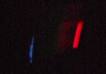
The I moved on to spectra tubes. Above one line from hydrogen is simply missing - the camera sensor is insensitive to that one wavelength.

Mercury had a golden line that was green in the raw camera image. Auto-balancing the image in GIMP restored the golden line.

Mercury displaying many pairs of red lines, a pair of yellow lines (color distorted above), a pair of orange lines, and a pair of faint green lines.
I showed the students the camera images and used the inability of the camera to image some light bands as a starting off point for a lecture on the subtleties of color perception. Somewhere in there is a laboratory struggling to get out.


Comments
Post a Comment