RipStik in Physical Science: Linear Velocity

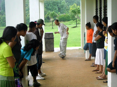
To demonstrate linear motion while retaining some modicum of attention span from my social media saturated students, I again rode a RipStik along the sidewalk in front of the laboratory. The activity is built around the linear relationship between time and distance for an object moving at a constant velocity. Thus my goal was to retain a constant velocity over the 36.8 meter distance.

In class I only wrote the time and distance data on the board, the following table was constructed later as part of my analysis of whether my speed was fairly constant. 

Pillar	Time (s)	Dist (m)	Vel (cm/s)	Acc (cm/s²)
one	0	0
two	3.86	4.6	1.19
three	6.89	9.2	1.52	0.11
four	9.64	13.8	1.67	0.06
five	12.45	18.4	1.64	-0.01
six	15.09	23	1.74	0.04
seven	17.84	27.6	1.67	-0.03
eight	20.47	32.2	1.75	0.03
nine	23.45	36.8	1.54	-0.07

A constant swizzle rate tends to generate acceleration early in the run, and I could feel the increase in the speed between pillars one and three. I started the run prior to pillar one, but only by about three meters, so I had not yet reached a constant speed as I passed pillar one.

During the summer I opted to delay the stopwatch start until the second pillar to provide a seven meter run prior to starting measurements, . This fall I returned to starting with the first pillar as zero. The small variations in speed are visually difficult to see and thus do not impact the finding of linearity for the system.

 

At the very end of the run I usually run off onto the asphalt walkway. A visitor to campus from Japan was standing in that location, so I had to stop swizzling and jump off immediately after the last column. The visitor had a somewhat bewildered expression on his face as I hurdled towards him.

The small increase in velocity among the first three pillars and the deceleration at the run's end can be seen above. Mid-run my speed held fairly steady, accelerations remained near zero. The overall average speed for the run was 1.57 m/s, with the linear regression best fit slope at 1.61 m/s.