5.3 Probability is relative frequency

Monday and section 5.1 opened with coverage of homework 4.4 and a working of the ball bounce statistics but using essay versus math for MHS. The board was balky and slow dealing with the large data set. Kept fighting against a copy and paste. By 9:20 I shifted into probability, distributing a penny to every student. A flip led to 8 heads and 9 tails. I flipped to make n even and landed a tenth tail. Why didn't we get 9 heads and 9 tails? Is the simulation broken again? No, random small variations away from 50/50 are expected. What isn't expected is 18 tails. Then I moved on into the core lecture including the unnin and thunnim, dice. The dice lecture was abbreviated as time constraints impinged on the presentation. I included a one side die in the lecture. 

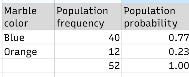
To demonstrate that relative frequency is probability and to show that sample values can only lead to conclusions about what the population values are not, not what they are, I used a mix of 40 blue marbles and 12 orange marbles. The marbles were placed in a bag and students drew one marble each in the blind from the bag.

The result was 62% blue and 38% orange. I then noted that we did not know how many marble were left in the bag. We know that the sample mean n is 21 marbles, but the population mean N remains unknown. Sample means do not inform us about population means. 

Then I noted that the only things we can be certain of is that 100% of the marbles are not blue and 100% of the marbles cannot be orange. We cannot know if there are perhaps some green marbles in the bag. We cannot know for certain what the actual proportions of blue and orange marbles are in the bag, or were before distribution. We can only say what we know not to be true, not what is true. 

I then ran an unexplained calculation of the 95% confidence interval for the blue marble proportion. I then told that class that I was confident that the population blue probability was within 22% of 62%, between 40% and 84%. And I told the class I could be wrong. In statistics one has to choose how wrong one is willing to be. One cannot always be right. How often do you want to be wrong? Never? Then you cannot be a statistician. 

I explained that I know I have at least a 5% risk of being wrong when I say the true proportion is between 40% and 84%. Of course I am either 100% right or 100% wrong, but over the long haul my estimate should be right 95% of the time. I left the mechanics of my calculation unexplained. 

At this point there were five orange marbles left in the bag. I dumped the bag into a box and showed the class the box with the remaining marbles. 

I noted that our sample data was incorrect. There were only 12 orange marbles but 8 + 5 is 13, not 12. So an error was made in the sampling phase. And this happens in statistics. Sampling errors and biases are always a possibility in statistics, although one tries to eliminate them as much as possible.

I also showed that the 77% was within the range I had calculated. So this time I was right - by calculating a range rather than a specific value, I was correct. The unequal distribution actually works better than the four way equal distribution allowing for more clarity in how the sample values do not match the population values. Although I had been aiming for a 70/30 split, the 77/23 split worked better in some ways.