Acceleration day one
Monday I tested a new approach to the opening RipStik acceleration run. Taking the three meter concept into week three I added only a 1.5 meter marker between 0 and 3 meters. Then I aimed to remain slow into the 3 meters marker, minimizing acceleration, possibly not accelerating except for the post push off at the start.


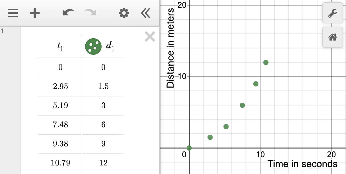
In class I chose to time the acceleration run myself, although I did bring along additional timers. The easier acceleration meant less concentration on remaining on the board. I suspect my times would be more internally consistent as well. In class the first 1.5 meters averaged 0.6 m/s. One student surmised that this might be a parabola.


Ahead of class I tested the concept and the result was no less reasonable than the prior terms where I used an increasing set of distances. I knew that there was a minimum stable speed down around 0.5 m/s below which two factors come into play. One is that the board is much harder to balance on - a stability issue. The other is that the board "stalls" on the smallest surface imperfection below around 0.5 m/s, the board simply has no momentum, the relative force of surface imperfections and friction are sufficient to stop a board moving below 0.5 m/s. That means a smooth increase to 0.5 m/s is not feasible, not possible.
The test run well supported my experience that speeds below 0.5 m/s are hard to sustain. The opening 1.5 meters on the test run clocked in at 0.51 m/s. Essentially I waited until three meters before I started actively working on accelerating. Even with no conscious attempt to accelerate until after the three meter mark, the board still rose to 0.67 m/s for the second 1.5 meters of the run.
This approach of not accelerating until three and then accelerating far less aggressively than I have done in the past allowed me to take the acceleration out the 12 meters and still only be at a speed of 2.13 m/s, well within my running speed range.
I started in the classroom by seeking predictions as to what the data would look like on a graph. Then the class moved to the sidewalk.


I then showed that this was a reasonable model. I brought along a poster pad and recorded the data and the equation on the poster pad. I noted that while the line goes through the points nicely enough, we really did not have evidence of what was happening to the left of the y-axis.

I then showed that an exponential function would also fit the data, differing only in the left tail. I used this to explain that this happens in physics research too: two models both fit data. Deciding which model is correct requires more data. So I said that on Wednesday we would look for data to decide between the two models.
The new approach of a deliberately slow acceleration with no effort before the 3 meter mark and taking the system out to 12 meters worked better than I expected, better than I hoped. This was a natural progression from using only three meter markers last week. I am always surprised when I eke out any kind of reasonable improvement in such a multi-year demonstration.
Comments
Post a Comment