Acceleration day two

Monday had been spent entirely out on the sidewalk using only a poster pad and a sketch of an argument that the shape was parabolic. Tuesday I started on the sidewalk with premarked distances of 3, 6, 9, 10, and 11 meters on the upslope into the Learning Resource Center.

Five stopwatches were handed out and three runs were made consecutively I then asked for a data from two of the runs. 

Desmos

I entered the raw data in the field for the two runs but did not run a regression. I could see that the second run was reasonably symmetric and decided that would do for the rest of the lecture.

This approach of a cold open in the field brought the class to the classroom by 12:14. This is the reverse order deployed in fall 2022 where I started with theory in the classroom to predict what would be seen. That approach brought the class to the sidewalk at 12:30. I think this sequence this term works better as the data provides numeric values for the quadratic equation.

The data was sketch onto the board on the left. A note was made that the time versus distance graph is not a graph of my path over the ground. My path over the ground was a straight up and back, drawn in red above. Then I argued that I was going to mash up last week's linear velocity equation d = vt with Monday's d = ½at² equation by adding them. I noted that there could be a d₀ starting distance, but that was zero again today. 

When I plug this into Desmos with subscripts adjusted to reflect the second table, I obtain a v₀ of 2.83 meters per second as I crossed the starting line. I showed where vee naught was on the graph. I then rewrote the equation as y = -0.225x²+2.83x+0 and put y = ax²+bx+c under that. 

The opened the path to explaining that quadratics encountered in the wild do not usually factor, thus spending time learning to factor in math classes was not productive nor useful activity. 

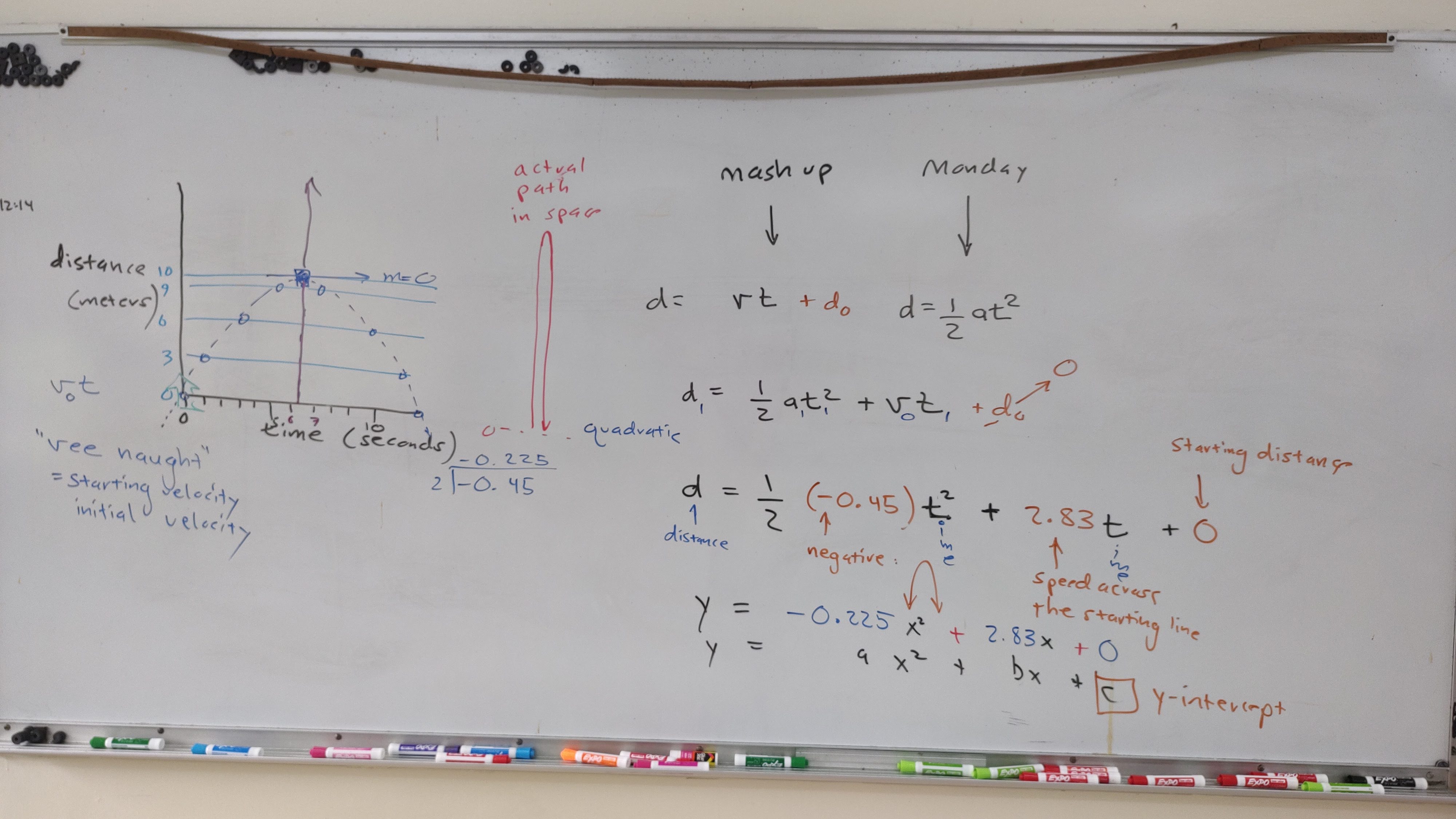
I then segued into covering the slope of the equation. I then showed that at t₂=0 the slope is 2.83 m/s as expected. I noted that the sketch of the graph on the board suggested a slope of zero up around six to seven seconds. Setting the slope equal to zero and solving for the time resulted in an answer of 6.29 seconds - between six and seven seconds. At twice that time (the curve is symmetric) the RipStik went back through the starting line at -2.83 m/s. 

Quadratic equations have a slope and intercept, but the slope is an equation. 

I wrapped up with a brief set of integrations and an explanation that this was the realm of calculus. I argue that it does no harm to see things one might not understand.