MS 150 Statistics class on nominal histograms began with 14 students. I handed out slips of blank paper to the students and asked them to write down their favorite color. Upon collecting the slips there were five blue, five black, two green, one gray, and one aqua. I wrote these down in a column on the whiteboard in order as color words. I noted that the sample size n was 14. I asked the class what was the level of measurement. One student suggested that the level was nominal, which is correct. This is qualitative, discrete, nominal level data. The data are the color words.
I then asked what the mode was for the data. The students saw the tie between blue and black, which is confusing. I explained that there is no mode - there is no one single data value that occurs more frequently. The data is, in some sense, bimodal: there are two modes, blue and black. A student entered and as she walked in I asked her what her favorite color is. She replied, "Gray." Shortly thereafter another student arrived at class and I asked her. "Blue," she responded. This brought the sample size to 16 and made blue the mode.
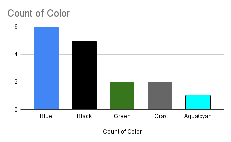
I then selected the column of color names and clicked on the chart wizard. Google Sheets does not balk at lists of words where repetition occurs. Google Sheets produced a pie chart of the data. I then changed to a column chart, as seen above after some custom coloring of the individual columns.
Referencing the column chart, I then produced the frequency table seen on the right above. I noted that the sum of the frequencies is the sample size. I again asked about the mode and a couple students said "two." This is the most common error students make in reading a frequency table. The mistake is thinking of the frequency column as the data. The data are the values in the first column. The most frequent is literally the most frequently occurring data value and is thus the data value corresponding to the maximum value in the second column. The mode is still blue with six instances of blue.
I used the frequency table to produce a pie chart. The pie chart provided the relative frequencies. The slices were custom colored to match the color word. The relative frequency was also calculated by a formula using a mixed relative and absolute address to keep the denominator locked on the sample size n.
I then wrapped up the class by noting that I had expected blue over black, green underneath, from the moment I had dressed for work that morning.
Blue shirt over black pants, green t-shirt, gray shoes. Blue over black, green under, and gray below. The order chosen by the class. How did I predict this? Magic? Future sight?
Well, actually, I had only predicted blue over black, green underneath. The gray shoes were not a deliberate choice that morning. This provides an opening to talk about the use of statistics in making predictions. I explained that while I do not know what color any one student will choose, for a large enough sample size I can predict the likely rank order of the colors. Sometimes I will be wrong. But I will usually only be wrong in the details: like black besting blue. I will still be roughly correct. I also explained that being wrong is part and parcel of doing statistics. One has to be comfortable with being wrong. If you like always being right, or have a driving need to be perfect, statistics is not the field for you.

My choice of clothes was driven by the
table above. 1456 students in MS 150 Statistics since summer 2007 have shared their favorite color. Blue holds the lead, followed by black, and green. I lack red shoes, and I could have chosen my white running shoes, but I went with the gray shoes that morning. Blue and black are almost always in the top two slots, with blue edging out black. And while blue is in the lead by 39 votes, blue has come out on top of black only 46% of the time. 43% of the time black tops blue. And 11% of the time blue and black tie, as was the situation with 14 students at the start of class. Choosing blue over black is close to a 50/50 shot at being right in small sample sizes. Blue does have an edge, hence I run with blue over black. Should that sequence ever overturn at the population level, then I would wear a black shirt and blue pants.

There are terms when another color comes out on top - sections sizes are small. In the fall of 2019 in the 9:00 section red took the top slot. And while I could not rescue my choice of black underneath, by combining the earlier 8:00 section results I could argue that I had to run with blue on top: 10 blue to 5 black and 8 red.
Over the years red remains the color most likely to alter the popularity rank order. Red is the state sports color for Yap state and the village sports color for Madolenihmw on Pohnpei. Madolenihmw possesses a strong sense of village based pride and this carries over into color choices. A section with spirit filled students from Yap and Madolenihmw can push red to the top. Brown is fairly steep drop below red. Brown has been number two in at least one term, but brown has never taken the top slot in a section.
In wrapping up I pointed out that I have had 1456 students in my statistics class just since 2007, not including the online terms when this exercise was not possible. I have been teaching statistics at the college since 2000, so the number across all 22 years is higher. Going back to when I started teaching at the college in 1992 the number of students is somewhere north of 4000. This is why I do not remember names. When a student asks, "Do you remember me?" I probably cannot. Yes, some people are good at keeping track of thousands of faces and names. I, however, am not.


Comments
Post a Comment